CQL2 Filtering

This notebook demonstrates using pystac-client to filter STAC items with CQL2 as described in the STAC API Filter Extension.

Note: Not all STAC APIs support the Filter Extension. APIs advertise conformance by including https://api.stacspec.org/v1.0.0/item-search#filter in the conformsTo attribute of the root API.

import json

import geopandas as gpd
import pandas as pd

from pystac_client import Client

The first step as always with pystac-client is opening the catalog:

# STAC API root URL
URL = "https://planetarycomputer.microsoft.com/api/stac/v1"

catalog = Client.open(URL)

Initial Search Parameters

Here we set up some initial search parameters to use with the Client.search function. We are providing a maximum number of items to return (max_items), a collection to look within (collections), a geometry (intersects), and a datetime range (datetime).

# AOI around Delfzijl, in the north of The Netherlands
geom = {
    "type": "Polygon",
    "coordinates": [
        [
            [6.42425537109375, 53.174765470134616],
            [7.344360351562499, 53.174765470134616],
            [7.344360351562499, 53.67393435835391],
            [6.42425537109375, 53.67393435835391],
            [6.42425537109375, 53.174765470134616],
        ]
    ],
}

params = {
    "max_items": 100,
    "collections": "landsat-8-c2-l2",
    "intersects": geom,
    "datetime": "2018-01-01/2020-12-31",
}

Using Filters

In addition to the parameters described above in the following examples we will filter by Item properties (filter) using CQL2-JSON. Here is a little function that does the search constructs a GeoDataFrame of the results and then plots datetime vs eo:cloud_cover.

Remember that in this whole notebook we are only looking at STAC metadata, there is no part where we are reading the data itself.

def search_and_plot(filter):
    search = catalog.search(**params, filter=filter)

    gdf = gpd.GeoDataFrame.from_features(search.item_collection_as_dict())
    gdf["datetime"] = pd.to_datetime(gdf["datetime"])
    print(f"Found {len(gdf)} items")

    gdf.plot.line(x="datetime", y="eo:cloud_cover", title=json.dumps(filter))

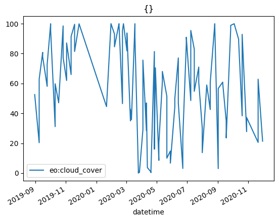
We can test out the function by passing an empty dict to do no filtering at all.

search_and_plot({})

Found 100 items

CQL2 Filters

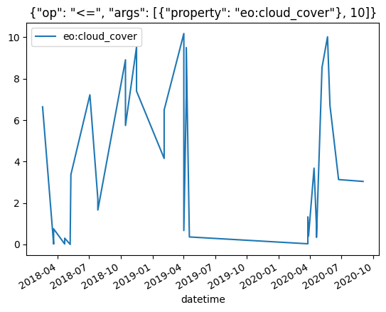
We will use eo:cloud_cover as an example and filter for all the STAC Items where eo:cloud_cover <= 10%.

filter = {"op": "<=", "args": [{"property": "eo:cloud_cover"}, 10]}

search_and_plot(filter)

Found 33 items

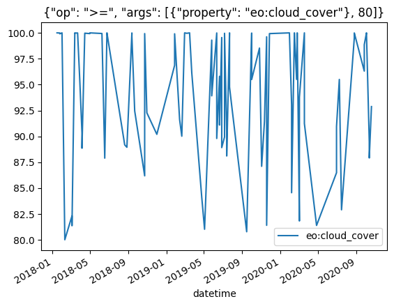
Next let’s look for all the STAC Items where eo:cloud_cover >= 80%.

filter = {"op": ">=", "args": [{"property": "eo:cloud_cover"}, 80]}

search_and_plot(filter)

Found 92 items

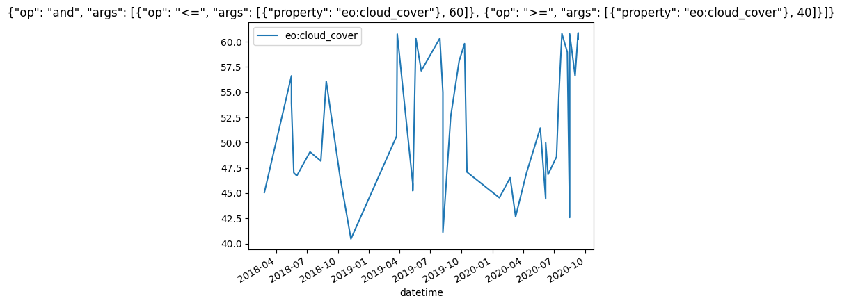
We can combine multiple CQL2 statements to express more complicated logic:

filter = {
    "op": "and",
    "args": [
        {"op": "<=", "args": [{"property": "eo:cloud_cover"}, 60]},
        {"op": ">=", "args": [{"property": "eo:cloud_cover"}, 40]},
    ],
}

search_and_plot(filter)

Found 41 items

You can see the power of this syntax. Indeed we can replace datetime and intersects from our original search parameters with a more complex CQL2 statement.

filter = {
    "op": "and",
    "args": [
        {"op": "s_intersects", "args": [{"property": "geometry"}, geom]},
        {"op": ">=", "args": [{"property": "datetime"}, "2018-01-01"]},
        {"op": "<=", "args": [{"property": "datetime"}, "2020-12-31"]},
        {"op": "<=", "args": [{"property": "eo:cloud_cover"}, 60]},
        {"op": ">=", "args": [{"property": "eo:cloud_cover"}, 40]},
    ],
}
search = catalog.search(max_items=100, collections="landsat-8-c2-l2", filter=filter)

print(f"Found {len(search.item_collection())} items")

Found 41 items

CQL2 Text

The examples above all use CQL2-json but pystac-client also supports passing filter as CQL2 text.

NOTE: As of right now in pystac-client if you use CQL2 text you need to change the search HTTP method to GET.

search = catalog.search(**params, method="GET", filter="eo:cloud_cover<=10")

print(f"Found {len(search.item_collection())} items")

Found 33 items

Just like CQL2 json, CQL2 text statements can be combined to express more complex logic:

search = catalog.search(
    **params, method="GET", filter="eo:cloud_cover<=60 and eo:cloud_cover>=40"
)

print(f"Found {len(search.item_collection())} items")

Found 41 items

Queryables

pystac-client provides a method for accessing all the arguments that can be used within CQL2 filters for a particular collection. These are provided as a json schema document, but for readability we are mostly interested in the names of the fields within properties.

NOTE: When getting the collection, you might notice that we use “landsat-c2-l2” as the collection id rather than “landsat-8-c2-l2”. This is because “landsat-8-c2-l2” doesn’t actually exist as a collection. It is just used in some places as a collection id on items. This is likely a remnant of some former setup in the Planetary Computer STAC.

collection = catalog.get_collection("landsat-c2-l2")
queryables = collection.get_queryables()

list(queryables["properties"].keys())

['id',
 'gsd',
 'created',
 'sci:doi',
 'datetime',
 'geometry',
 'platform',
 'proj:epsg',
 'instrument',
 'proj:shape',
 'description',
 'instruments',
 'end_datetime',
 'eo:cloud_cover',
 'proj:transform',
 'start_datetime',
 'view:off_nadir',
 'landsat:wrs_row',
 'landsat:scene_id',
 'landsat:wrs_path',
 'landsat:wrs_type',
 'view:sun_azimuth',
 'landsat:correction',
 'view:sun_elevation',
 'landsat:cloud_cover_land',
 'landsat:collection_number',
 'landsat:collection_category']

Read More

• For more involved CQL2 examples in a STAC context read the STAC API Filter Extension Examples

• For examples of all the different CQL2 operations take a look at the playground on the CQL2-rs docs.